Conditional Cell Formatting in Excel 2007/2010

If you are working on a spreadsheet and want to be able to quickly see differences in numbers at a glance, you should use the new Conditional Cell Formatting in Excel 2007/2010. With this you can change the background of a cell based on the data in the cell, almost like an inline chart.
Using Conditional Formatting
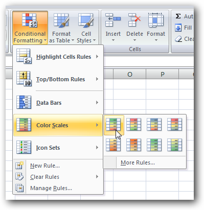
Once you select the cells that you want to format, you can find the Conditional Formatting drop-down on the ribbon, which gives you loads of pre-set rules to choose from, like color scales.

This will automatically color the items based on the range they are in…

You can also choose to use icons instead:

Reminds me of that commercial… more bars in more places…

You can also create your own rule to color only cells that fit within a certain range, or greater than a certain number.

This rule will only color cells greater than a certain amount, with the color you specify.

This can be very useful, and you should note that you can apply a second rule to the same range. For instance, I added a second rule that colored items larger than 2000 with green instead of red.

You can even create a completely customized rule by choosing the New Formatting Rule option.

If you’ve applied too many rules and want to start over, just select the cells and use the Clear Rules option to remove all the formatting.

This is one of those really useful features that make Office 2007 a lot better than the prior versions.